PSTAT 5A: Lecture 21
Intro to Statistical Modeling, and Correlation
2024-07-25
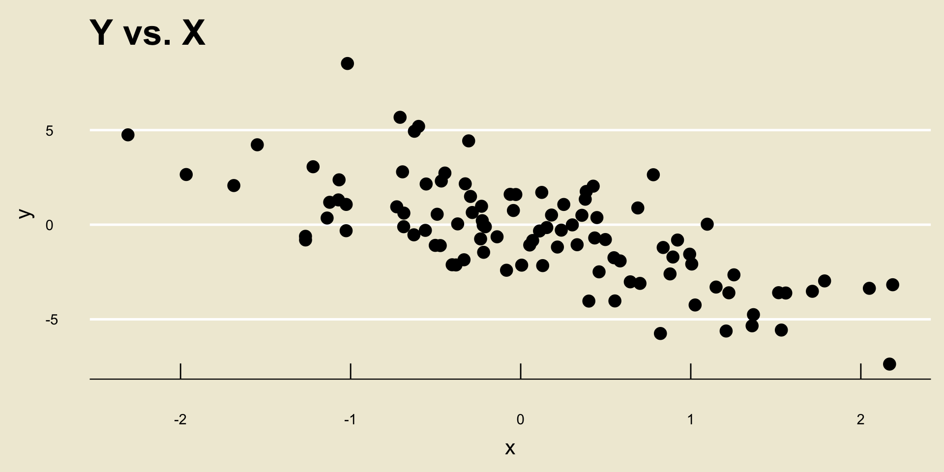
- Linear Negative Association:
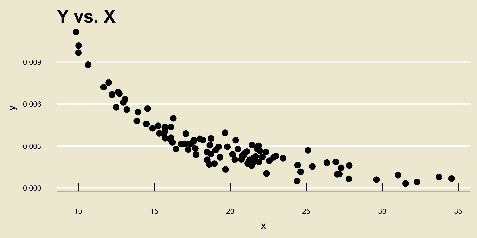
- Nonlinear Negative Association:
- Linear Positive Association:

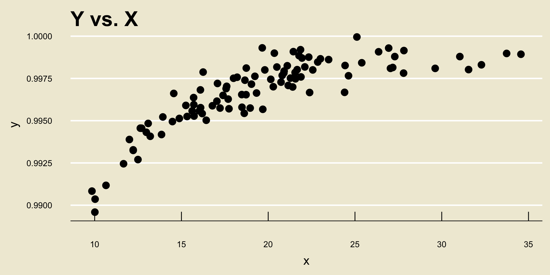
- Nonlinear Positive Association:
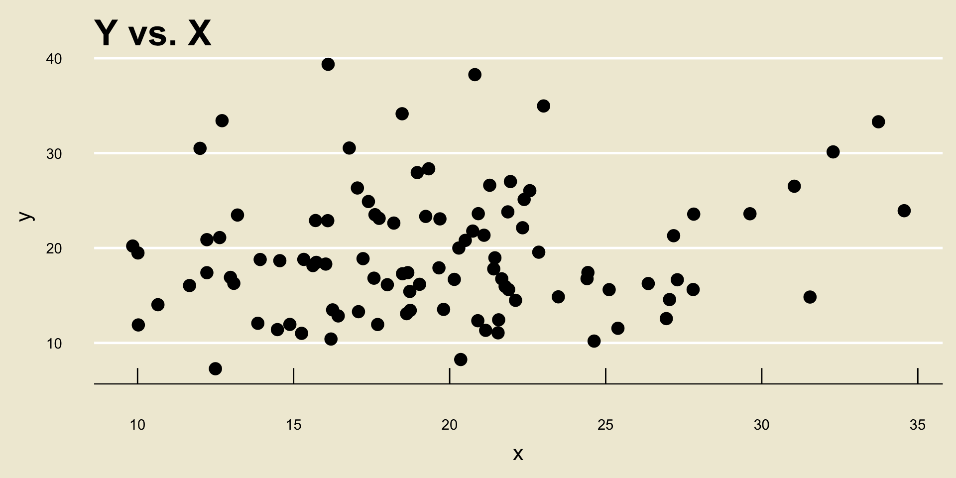
No Relationship
- Sometimes, two variables will have no relationship at all:
Classification Problem
Another example is returning to our Penguins dataset. Here is a scatterplot of flipper length by bill length:

This is clearly very linear but it’s missing an additional element.
Classification Problem

Strength of a Relationship
Now, before we delve into the mathematics and mechanics of model fitting, there is another thing we should be aware of.
As an example, consider the following two scatterplots:
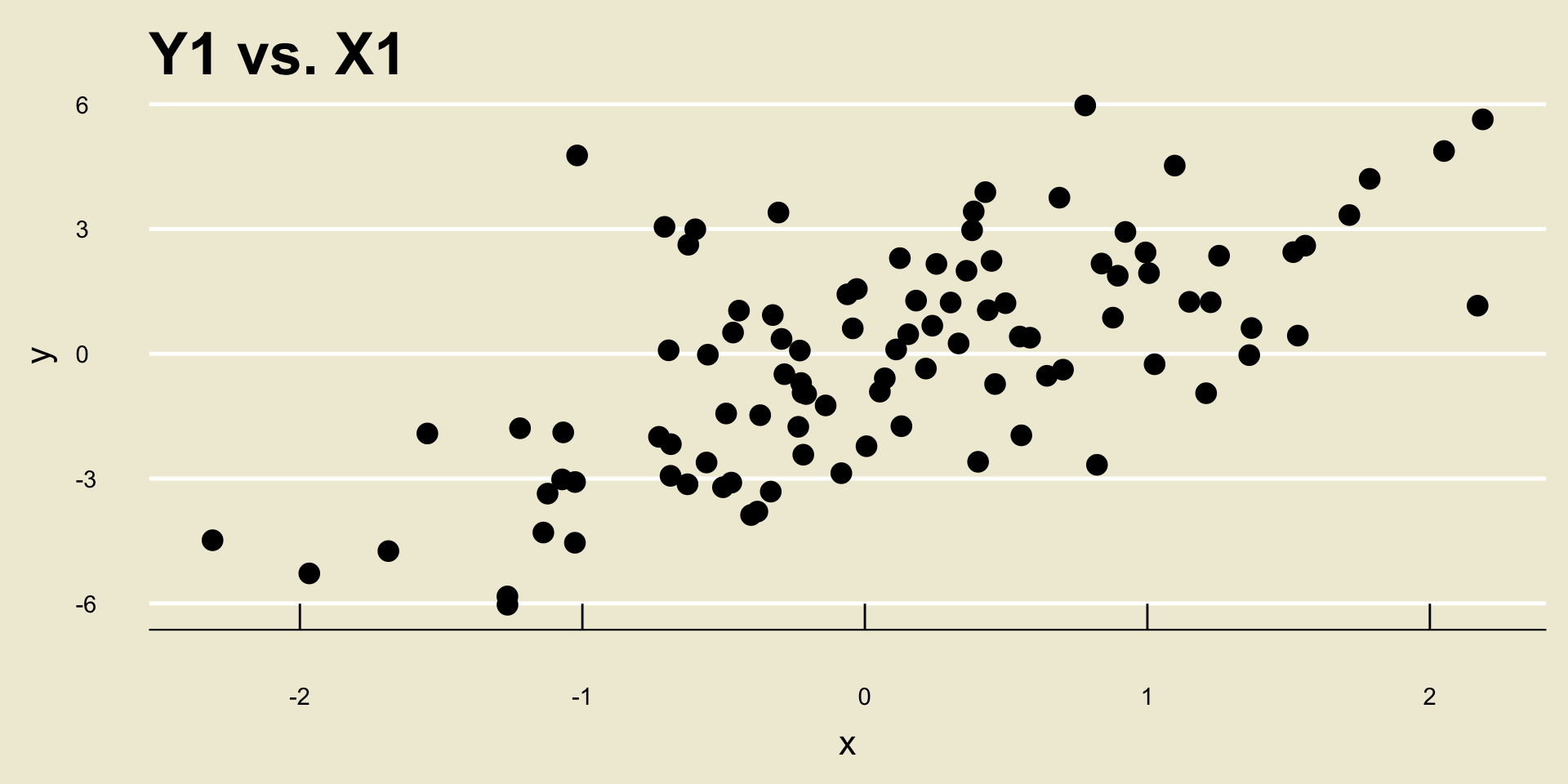
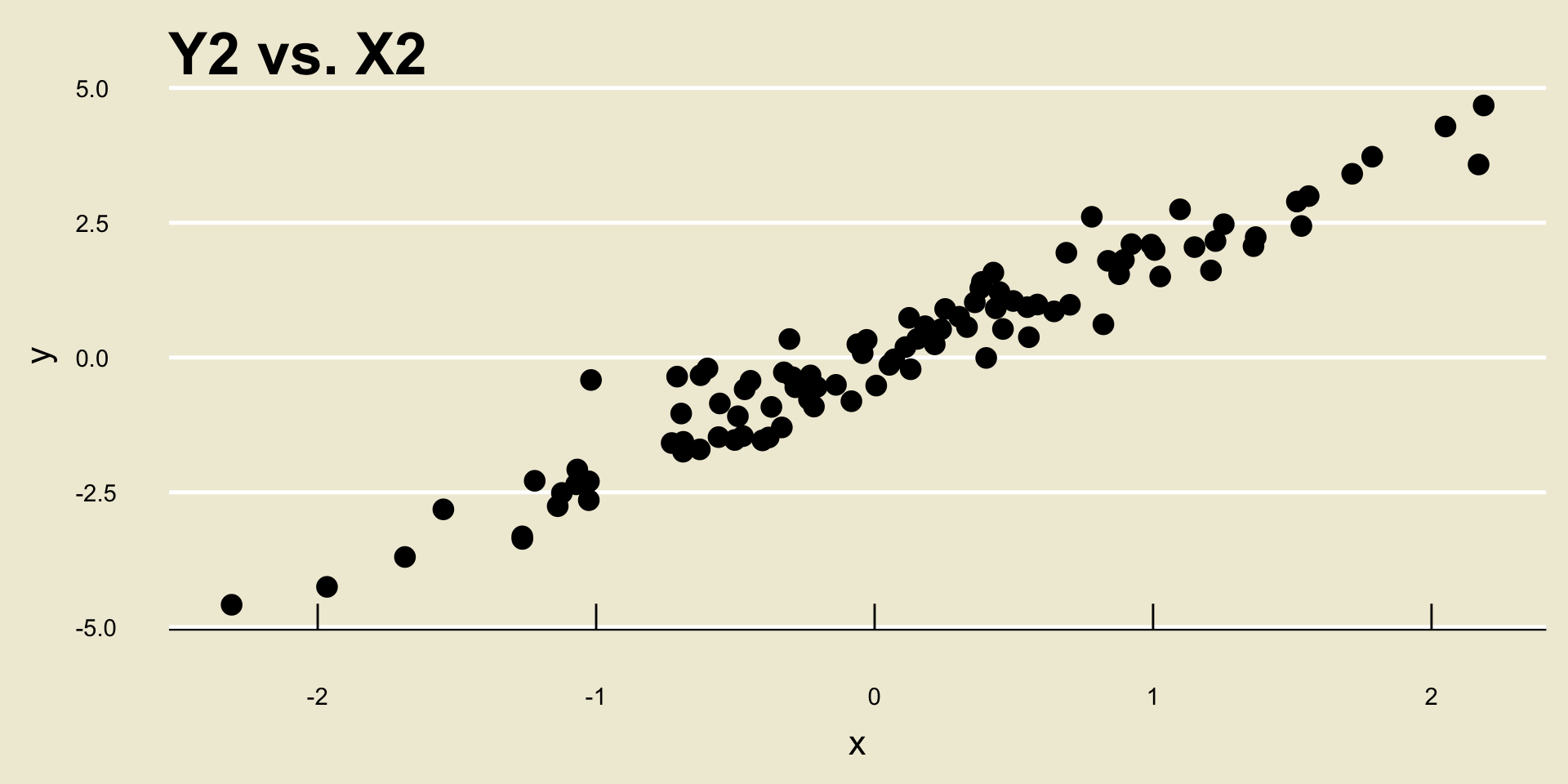
- Both scatterplots display a positive linear trend. However, the relationship between
Y2andX2seems to be “stronger” than the relationship betweenY1andX1, does it not?
Important Distinction
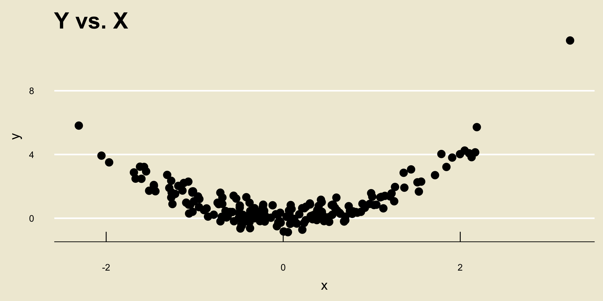
Now, something that is very important to mention is that r only quantifies linear relationships- it is very bad at quantifying nonlinear relationships.
For example, consider the following scatterplot:
Leadup
There is another thing to note about correlation.
Let’s see this by way of an example: consider the following two scatterplots:
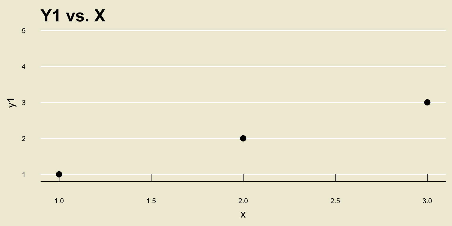
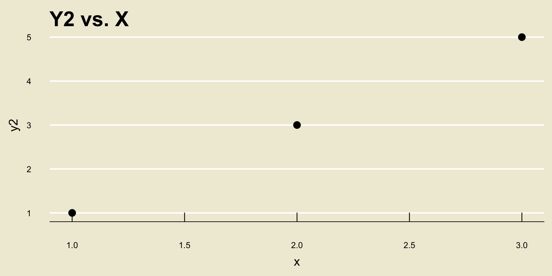
- Both cor(
X,Y1) and cor(X,Y2) are equal to 1, despite the fact that a one unit increase inxcorresponds to a different unit increase iny1as opposed toy2.
Regression Problem
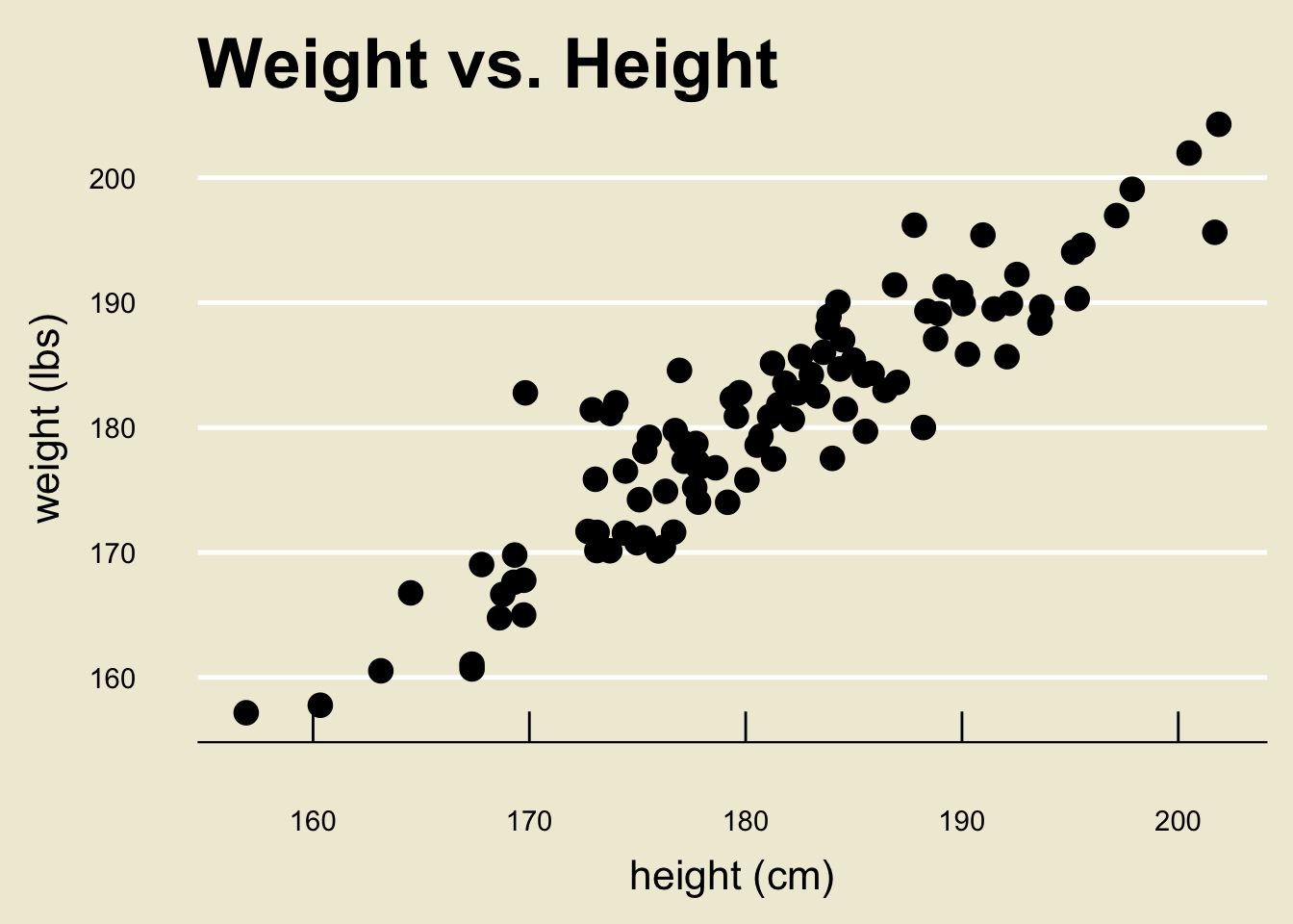
- As a concrete example, let’s examine a dataset that contains several measurements on heights and weights:

Height and Weight
- Okay, back to our height and weight example:
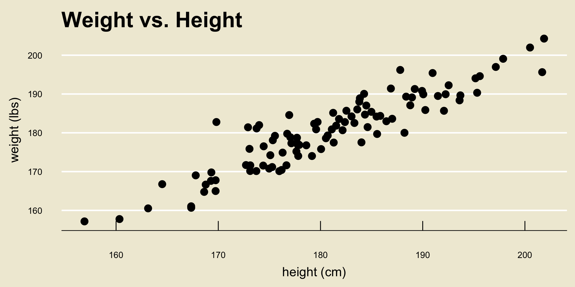
Height and Weight
The regression problem basically boils down to finding the line that best fits the data.
The specific line we will discuss in a bit is called the ordinary least squares line (or just OLS line):
Simple Linear Regression
- Here’s a visual way of thinking about this. Consider the following scatterplot:
![]()
Goals
- We are assuming that there exists some true linear relationship (i.e. some “fit”) between
yandx. But, because of natural variability due to randomness, we cannot figure out exactly what the true relationship is.

Goals
- Finding the “best” estimate of the signal function is, therefore, akin to finding the line that “best” fits the data.

Residuals
- The ith residual is defined to be the quantity \(e_i\) below:

- RSS is then just \(\displaystyle \mathrm{RSS} = \sum_{i=1}^{n} e_i^2\)
Example

Example
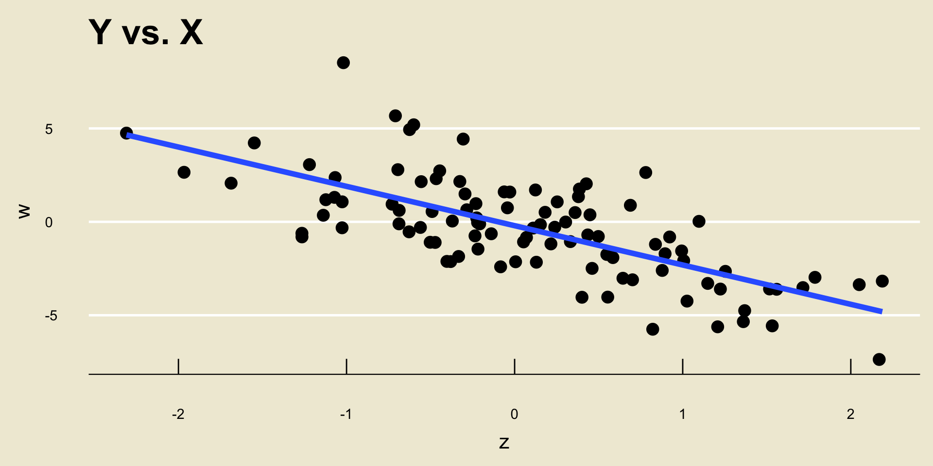
\(\widehat{\beta_0} =\) -0.2056061; \(\widehat{\beta_1} =\) -2.1049432.
I.e. the equation of the line in blue is -0.2056061 + -2.1049432 *
x.
Fitted Values
- Let’s return to our cartoon picture of OLS regression:
Fitted Values
- Notice that each point in our dataset (i.e. the blue points) have a corresponding point on the OLS regression line:

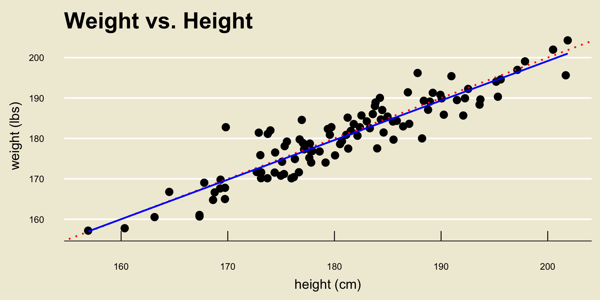
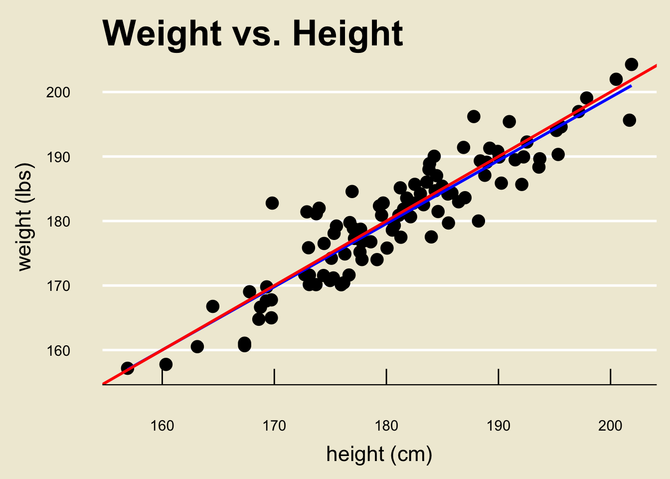
Back to height and weight
- Before we work through the math once, let’s apply this technique to the height and weight data from before.
Back to height and weight
- Using a computer software, the OLS regression line can be found to be:
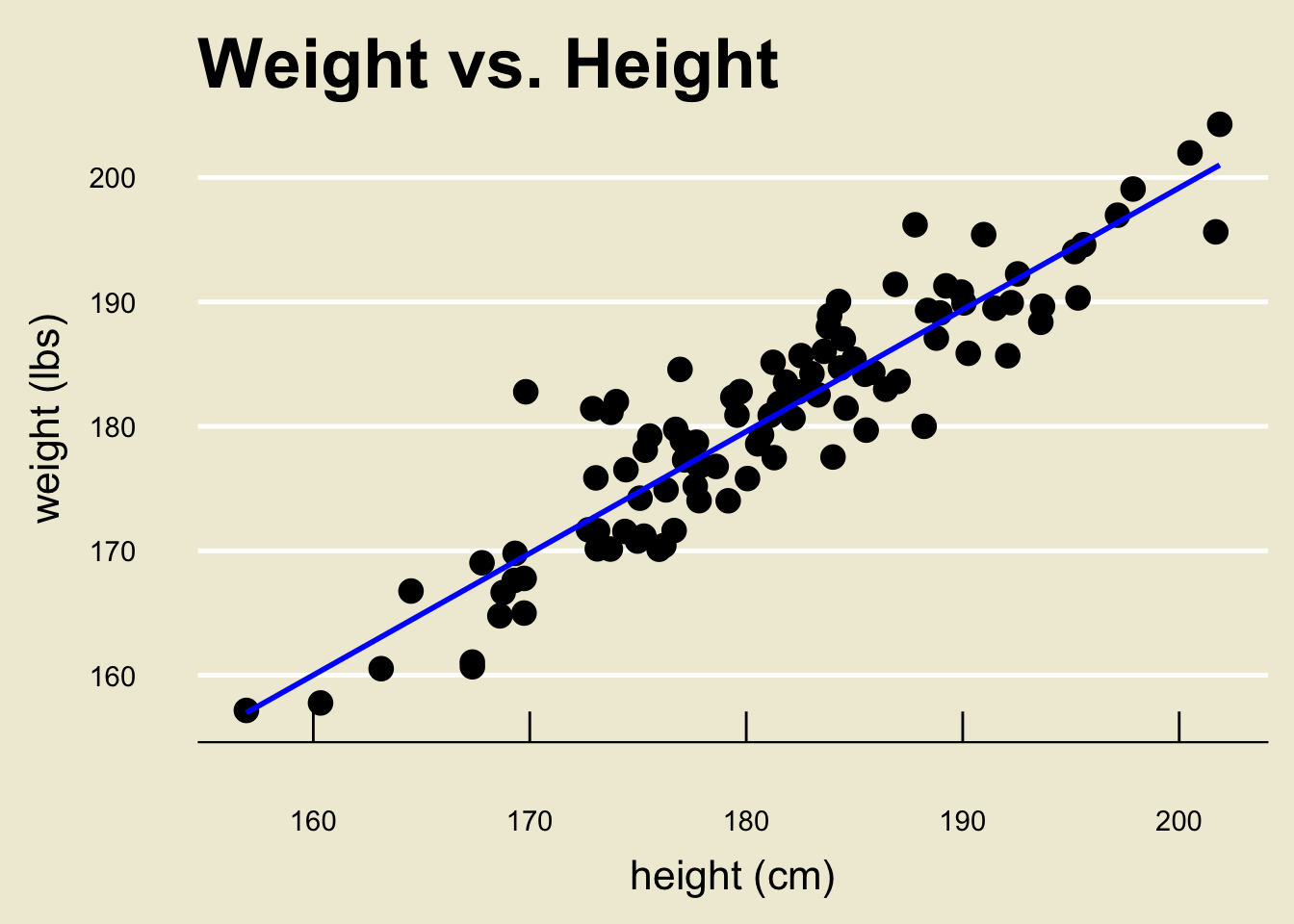
- Specifically, \(\widehat{\beta_0} =\) 3.366744 and \(\widehat{\beta_1} =\) 0.9790114
- We will return to the notion of fitted values in a bit.
\[ \widehat{\texttt{weight}} = 3.367 + 0.979 \cdot \texttt{height} \]
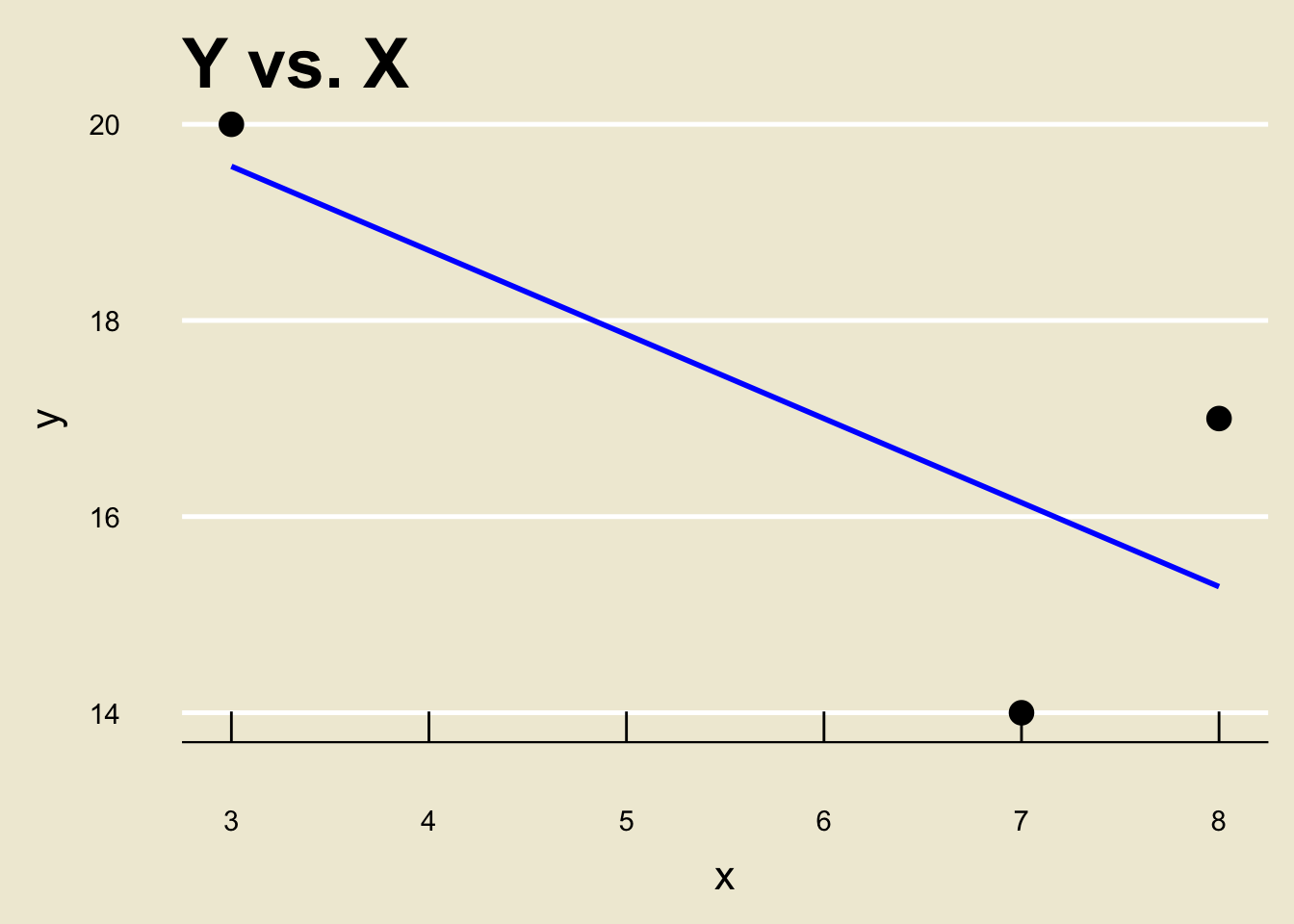
\[ \widehat{y} = \frac{1}{7} ( 155 - 6 x ) \]
Next Time
- Next time, we’ll discuss how to use the OLS regression line to make predictions.